2020 ATAC-seq analysis
ATAC-seq最新处理流程
2020 ATAC-seq analysis
一、ATAC-seq个性化的conda environment的搭建
1、git clone
git clone文章中提到的atac-seq-pipeline (里面有你接下来分析所需要的绝大部分东西。另外一定要去看README.md,这个文档会告诉你分析ATAC-seq需要做些准备,进行些什么工作。)
1 | $ cd ~/ATAC |
2、环境搭建
(1)conda base environment搭建
1 | #一路yes下去 |
(2)失活掉base conda environment自动激活的设置
1 | $ conda config --set auto_activate_base false |
(3)安装pipeline’s conda environment
!?你是不是充满了疑问!?下面的两个shell脚本哪里冒出来的,干什么用的。不要忘了,我们第一步git clone了这个atac-seq-pipeline呢!这两个脚本就是就是来源于这个clone下来的pipeline的。
1 | # 网不给力的朋友,比如说我,这一部就是整个分析流程的限速步骤!!!网络给力这一步也需要花一些时间,读一下两个shell文件就知道为什么啦。 |
(4)激活安装的conda环境
1 | $ conda activate encode-atac-seq-pipeline |
(5)查看所有的conda环境
1 | conda env list |
我们会看到有一个基于python2的环境,没有标明python版本的那个encode-atac-seq-pipeline是基于python3的。有些软件是要基于特定版本的python运行的。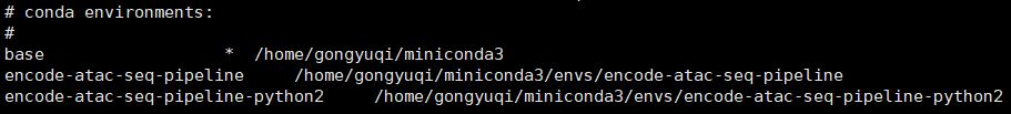
二、数据下载
1 | #一次性下载所有的......_1.fastq.gz和......_2.fastq.gz样本 |
三、bowtie2比对
1、 fastqc+multiqc查看原始数据的质量情况
1 | conda install -y fastqc multiqc |
multiqc结果表明原始数据质量已经很好了,完全没有adaptor残留,连PCR重复都是勉强过关的。per base sequence content和kmer content两项指标不合格,但是并不会对后续的比对造成多大的负面影响,同时这两项指标通过过滤软件的处理可能并不会后得到改善。这样的数据其实可以直接比对的。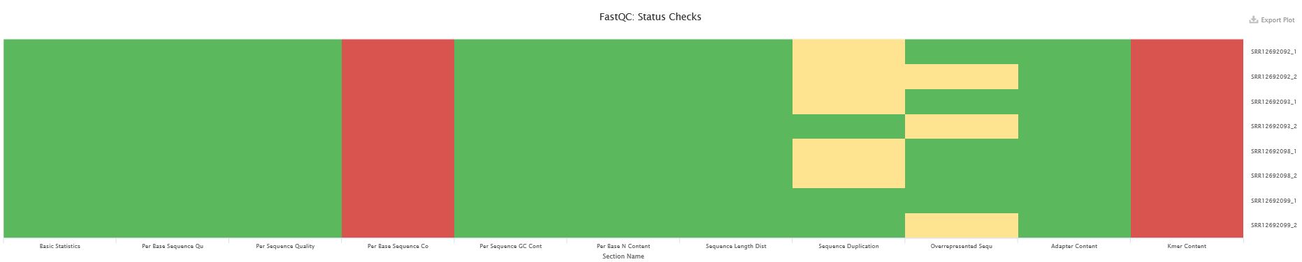
2、 过滤低质量的reads
(如果原始数据需要进行过滤处理,那么走下面这个过滤流程,我们这里就不过滤了)
1 | nohup cat rawdata.txt|while read id |
3、 比对参考基因组
比对
1
2
3
4
5
6
7
8nohup cat sample.txt | while read id
do
arr=(${id})
fq1=${arr[0]}
fq2=${arr[1]}
sample=${fq1%%_*}.sort.bam
bowtie2 --very-sensitive -X2000 --mm --threads 8 -x /home/gongyuqi/ref/mm10/index/mm10 -1 $fq1 -2 $fq2|samtools sort -O bam -@ 8 - -o ../align/$sample
done &比对情况统计及查看
1
2
3
4
5ls *.bam | while read id
do
nohup samtools flagstat -@ 4 $id > ${id%%.*}.stat &
done
ls *.stat | while read id; do cat $id | grep "mapped (";done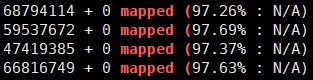
生成bam文件的索引文件
1
nohup ls *sort.bam|while read id; do samtools index -@ 10 $id;done &
四、PCR去除重及质控制
1、初步过滤
#=============================
#Remove unmapped, mate unmapped
#not primary alignment, reads failing platform
#Only keep properly paired reads
#Obtain name sorted BAM file
#=============================================
1 | #fixmate要求输入的bam文件按名称排序,所以第一步初步过滤后要按reads名称排序一下 |
2、进一步
#===============================================
#Remove orphan reads (pair was removed)
#and read pairs mapping to different chromosomes
#Obtain position sorted BAM
#===============================================
1 | #多个样本写循环 |
3、标记PCR重复
#===============
#Mark duplicates
#===============
1 | MARKDUP=/home/gongyuqi/miniconda3/envs/encode-atac-seq-pipeline/share/picard-2.20.7-0/picard.jar |
4、去除PCR重复、建立索引文件、按name排序的bam文件、质控文件
#============================
#Remove duplicates
#Index final position sorted BAM
#Create final name sorted BAM
#============================
1 | #多个样本写循环 |
5、测序文库复杂度的检验
#=============================
#Compute library complexity
#=============================
#Sort by name
#convert to bedPE and obtain fragment coordinates
#sort by position and strand
#Obtain unique count statistics
#================================================
1 | #多个样本写循环 |
Library complexity measures计算结果如下,…nodup.pbc.qc文件格式为:
TotalReadPairs
DistinctReadPairs
OneReadPair
TwoReadPairs
NRF=Distinct/Total
PBC1=OnePair/Distinct
PBC2=OnePair/TwoPair
针对NRF、PBC1、PBC2这几个指标,ENCODE官网提供的标准如下:
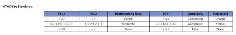
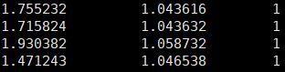
我们此次4个样本的分析结果显示这几个指标的值如下所示:
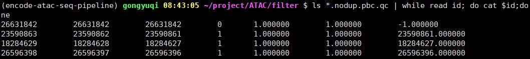
除了第一个样本(SRR12692092),其他样本计算结果显示NRF、PBC1、PBC2的值都非常完美,说明我们进行过滤和PCR去重的bam文件质量上没有问题,可以用于后续的分析。
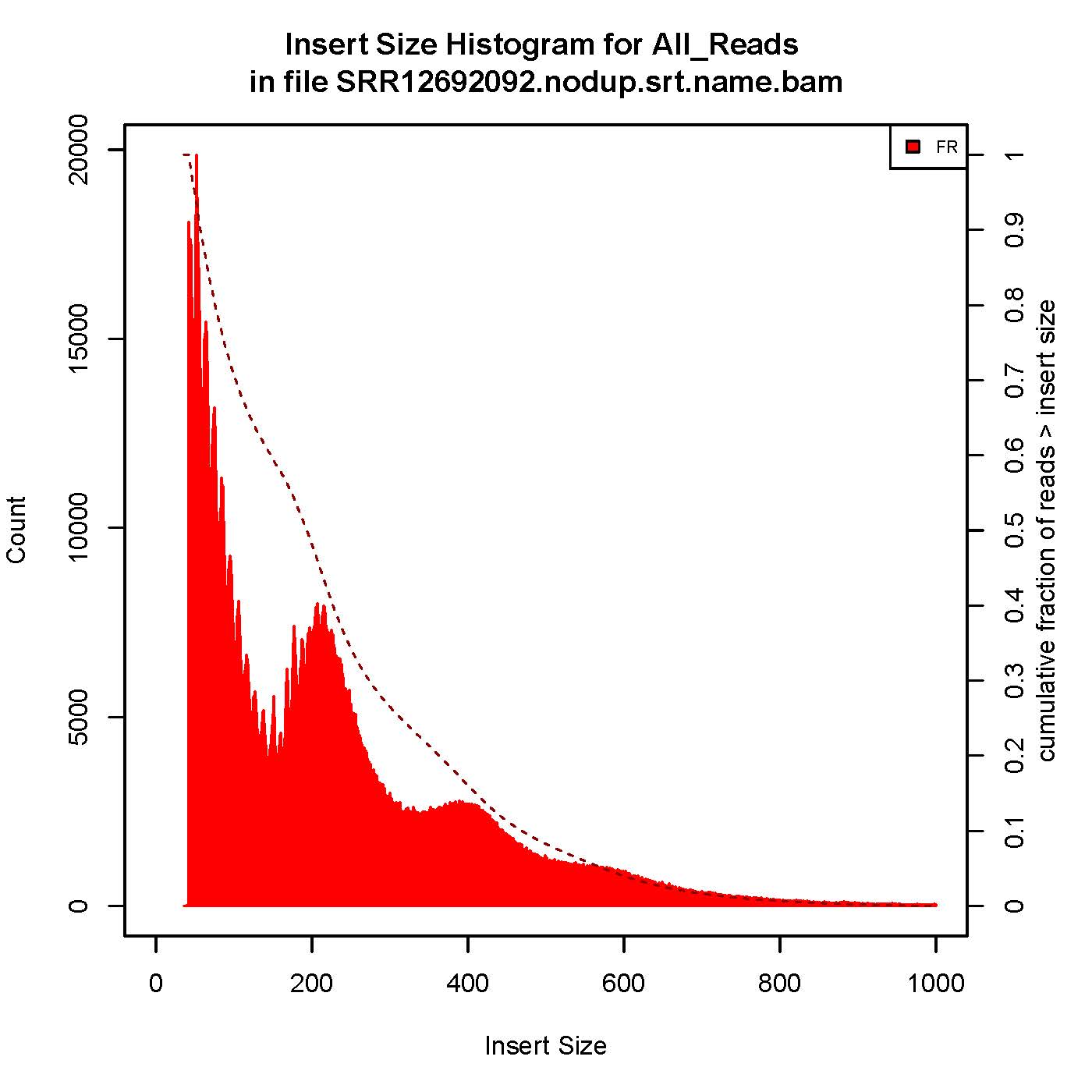
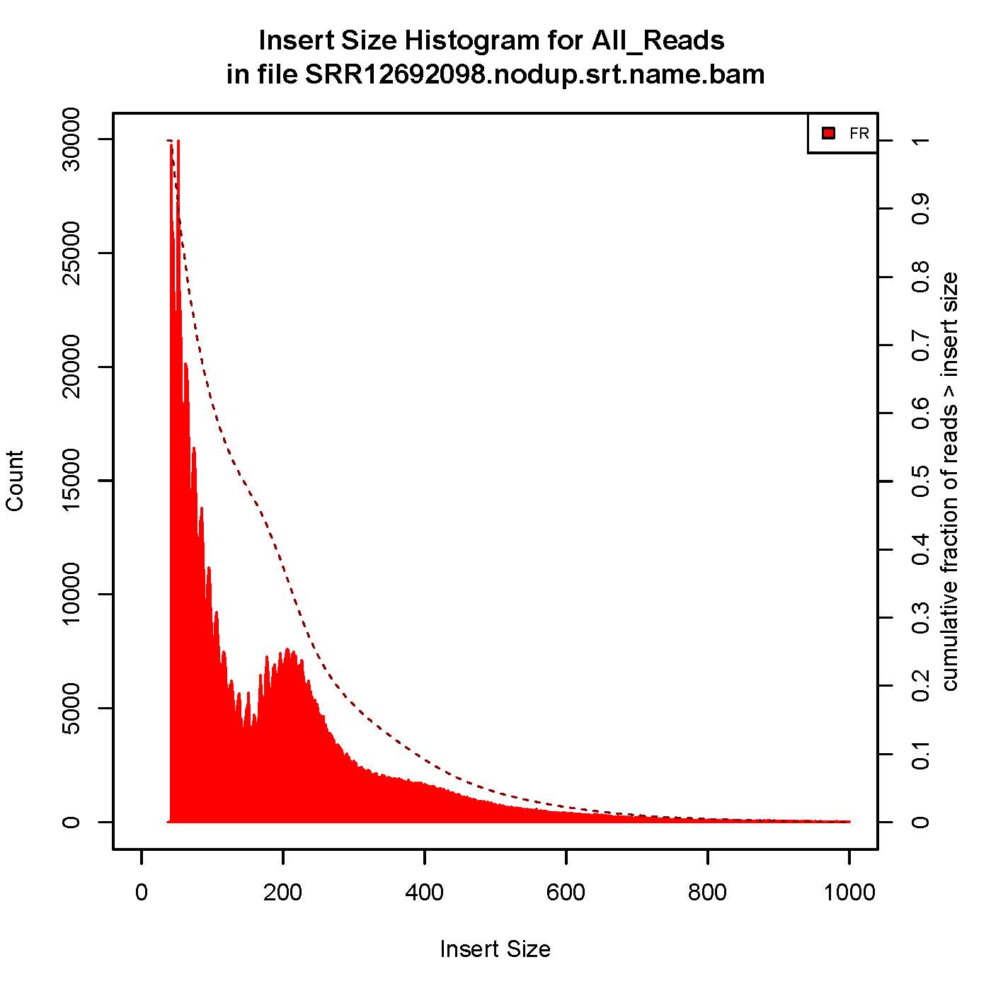
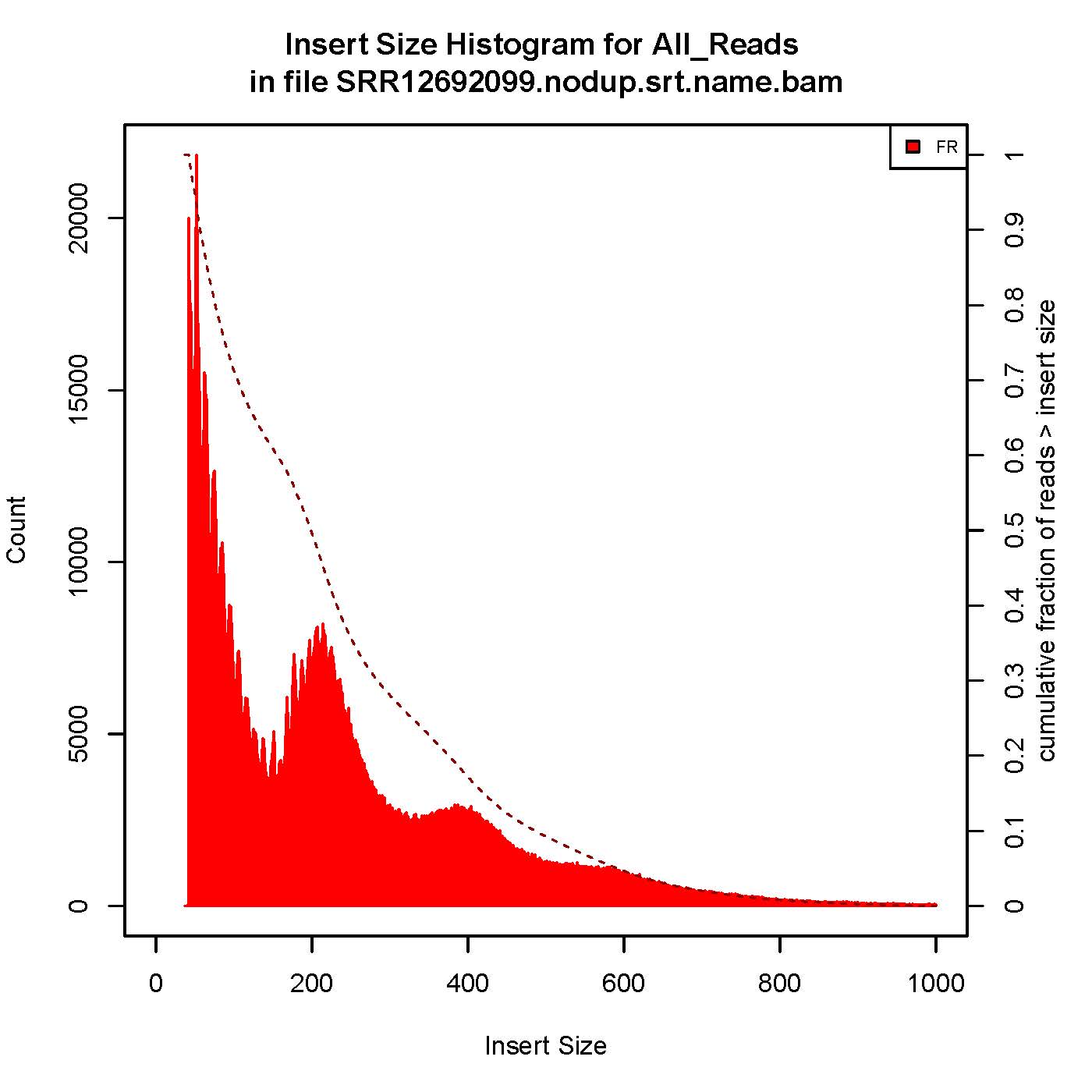
6、插入片段质控检测
| 用于评估ATAC/Chip实验质量好坏的一个重要指标 |
1 | #多个样本循环 |
成功的ATAC-seq实验会生成具有逐级递减和周期性的峰,对应无核小体区域(Nucleosome free region, NRF,100bp),单核区域(mono-nucleosome,200bp),双核区域(400bp),三核区域(600bp)。
本次结果显示样本质量OK

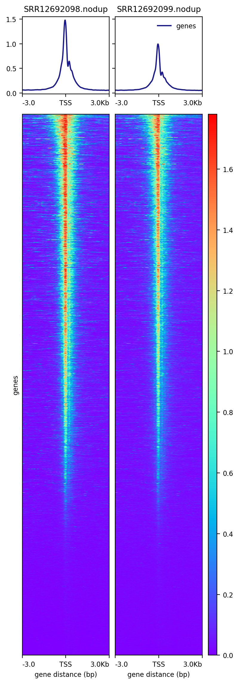
7、TSS富集
以BRM014-10uM_24h_wt样本为例,可视化peaks在基因组上的分布特征(TSS区域;TSS、gene-body、TSE区域)
- both -R and -S can accept multiple files
- UCSC官网下载小鼠参考基因组注释文件,详情参考:http://www.bio-info-trainee.com/2494.html
1 | #生成bw文件用于后续的computeMatrix |

五、生成tagAlign格式文件
1. Convert PE BAM to tagAlign
- 对于单端序列。直接用bed格式就可以;对于双端序列,推荐用bedpe格式。这两种格式都可以称之为tagAlign,可以作为macs的输入文件。
- tagAligen格式相比bam,文件大小会小很多,更加方便文件的读取。在转换得到tagAlign格式之后,我们就可以很容易的将坐标进行偏移
1 | nohup ls *nodup.srt.name.bam|while read id; do bedtools bamtobed -bedpe -mate1 -i $id | gzip -nc > ${id%%.*}.nodup.srt.name.bedpe.gz;done & |
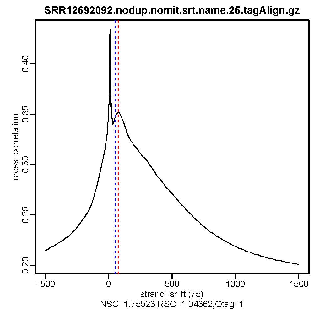
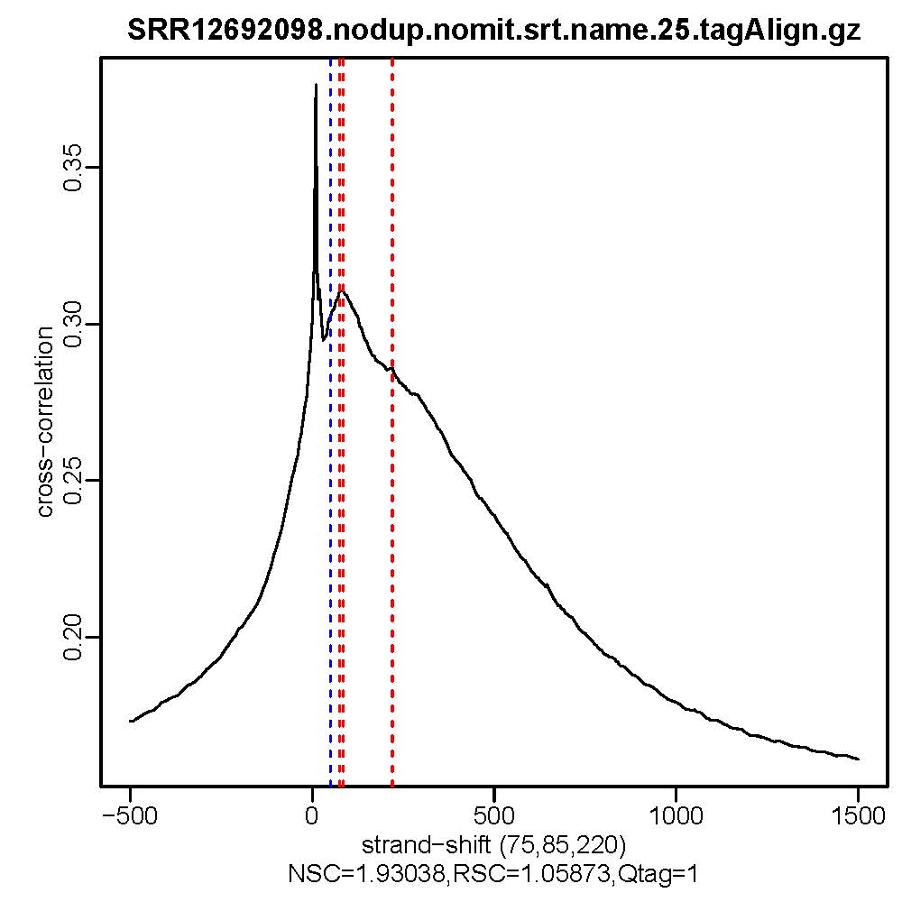
2. Stand Cross Correlation analysis
| 用于评估ATAC/Chip实验质量好坏的一个重要指标 |
1 | NREADS=25000000 |


- 质控结果解读
Normalized strand cross-correlation coefficent (NSC):NSC是最大交叉相关值除以背景交叉相关的比率(所有可能的链转移的最小交叉相关值)。NSC值越大表明富集效果越好,NSC值低于1.1表明较弱的富集,小于1表示无富集。NSC值稍微低于1.05,有较低的信噪比或很少的峰,这肯能是生物学真实现象,比如有的因子在特定组织类型中只有很少的结合位点;也可能确实是数据质量差。
Relative strand cross-correlation coefficient (RSC):RSC是片段长度相关值减去背景相关值除以phantom-peak相关值减去背景相关值。RSC的最小值可能是0,表示无信号;富集好的实验RSC值大于1;低于1表示质量低。
QualityTag: Quality tag based on thresholded RSC (codes: -2:veryLow,-1:Low,0:Medium,1:High,2:veryHigh)
查看交叉相关性质量评估结果,主要看NSC,RSC,Quality tag三个值,这三个值分别对应输出文件的第9列,第10列,第11列。
六、Call Peaks
1、去除线粒体基因的TagAlign格式文件进行shift操作,输入macs2软件去callpeak
1 | smooth_window=150 # default |
2、去除ENCODE列入黑名单的区域
去除黑名单的bed文件,用于后续的peaks注释
1
2
3
4
5
6
7BLACKLIST=/home/gongyuqi/project/ATAC/mm10.blacklist.bed.gz
#*_summits.bed为macs2软件callpeak的结果文件之一
nohup ls *_summits.bed | while read id; do bedtools intersect -a $id -b $BLACKLIST -v > ${id%%.*}_filt_blacklist.bed; done &
#查看过滤黑名单的区域前后的bed文件的peaks数
ls *summits.bed|while read id; do cat $id |wc -l >>summits.bed.txt;done
ls *summits_filt_blacklist.bed|while read id; do cat $id |wc -l >>summits_filt_blacklist.bed.txt;done
past summits.bed.txt summits_filt_blacklist.bed.txt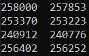
去除黑名单的narrowPeaks文件,用于后续的IDR评估
1
2
3
4
5
6
7
8
9
10
11
12#使用IDR需要先对MACS2的结果文件narrowPeak根据-log10(p-value)进行排序,-log10(p-value)在第八列。
# Sort by Col8 in descending order and replace long peak names in Column 4 with Peak_<peakRank>
#*_peaks.narrowPeak为macs2软件callpeak的结果文件之一
NPEAKS=300000
ls *_peaks.narrowPeak | while read id; do sort -k 8gr,8gr $id | awk 'BEGIN{OFS="\t"}{$4="Peak_"NR ; print $0}' | head -n ${NPEAKS} | gzip -nc > ${id%%_*}.narrowPeak.gz; done
BLACKLIST=../BLACKLIST/mm10.blacklist.bed.gz
#生成不压缩文件
ls *.narrowPeak.gz | while read id; do bedtools intersect -v -a $id -b ${BLACKLIST} | awk 'BEGIN{OFS="\t"} {if ($5>1000) $5=1000; print $0}' | grep -P 'chr[\dXY]+[ \t]' > ${id%%.*}.narrowPeak.filt_blacklist; done
#生成压缩文件
#ls *.narrowPeak.gz | while read id; do bedtools intersect -v -a $id -b ${BLACKLIST} | awk 'BEGIN{OFS="\t"} {if ($5>1000) $5=1000; print $0}' | grep -P 'chr[\dXY]+[ \t]' | gzip -nc > ${id%%.*}.narrowPeak.filt_blacklist.gz; done
3、Irreproducibility Discovery Rate (IDR)评估
| 用于评估重复样本间peaks一致性的重要指标 |

1 | nohup cat narrowPeak_sample.txt | while read id |
- DMSO_24h_wt (样本处理情况)
- SRR12692092.filt_blacklist.narrowPeak SRR12692093.filt_blacklist.narrowPeak
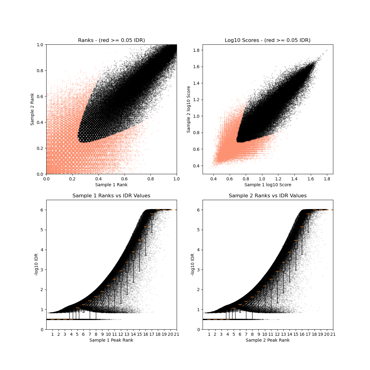
- 没有通过IDR阈值的显示为红色
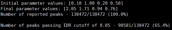
- BRM014-10uM_24h_wt (样本处理情况)
- SRR12692098.filt_blacklist.narrowPeak SRR12692099.filt_blacklist.narrowPeak
- 没有通过IDR阈值的显示为红色
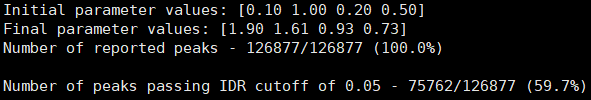

IDR评估会同时考虑peaks间的overlap和富集倍数的一致性。通过IDR阈值(0.05)的占比越大,说明重复样本间peaks一致性越好。从idr的分析结果看,我们的测试数据还可以的呢。
IDR评估相关参考资料:
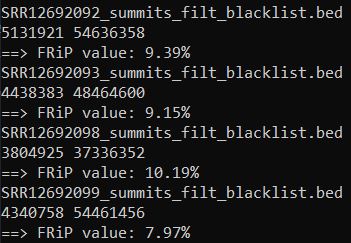
4、Fraction of reads in peaks (FRiP)评估
| 反映样本富集效果好坏的评价指标 |
1 | #生成bed文件 |
FRiP值在5%以上算比较好的。但也不绝对,这是个软阈值,可以作为一个参考。
FRiP评估相关参考资料:
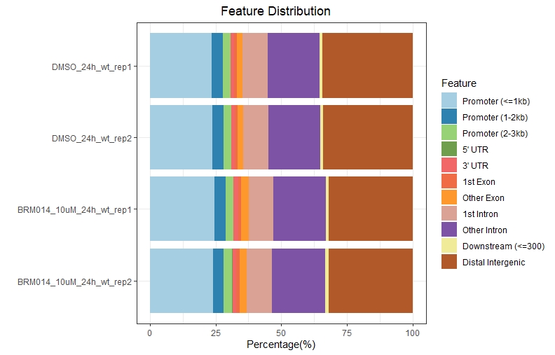
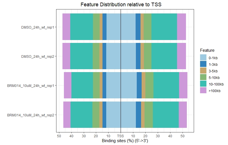
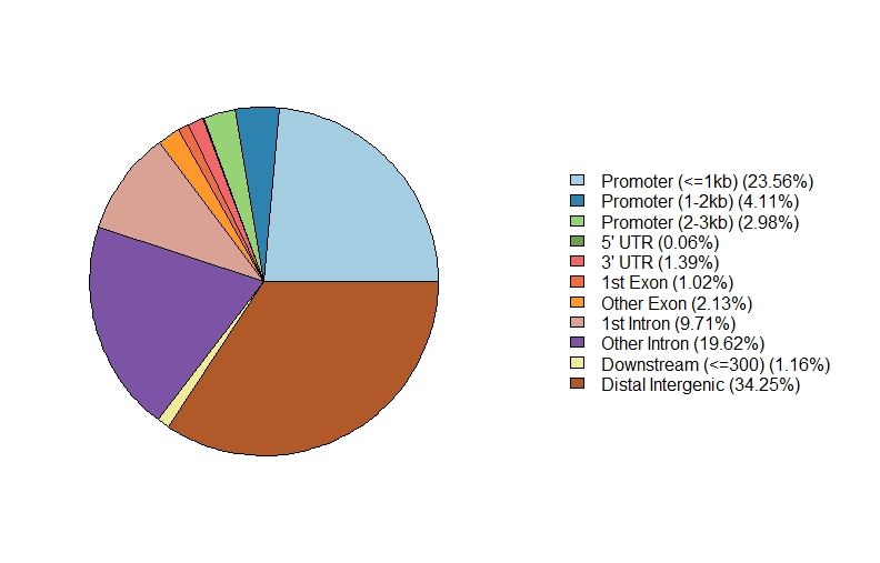
七、Peak annotation
1、Feature Distribution
1 | setwd("path to bed file") |
.jpeg)
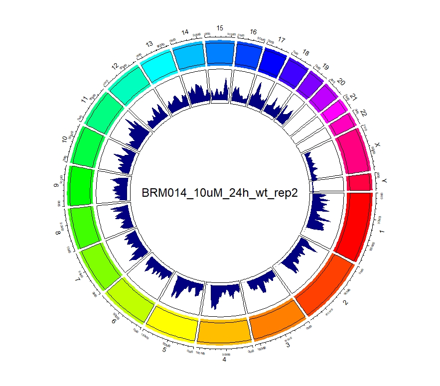
2、查看peaks在全基因组上的分布
1 | #输入文件的准备 |
看到这样的结果,第一反应就是————为什么两种处理情况下染色体开放程度那么像!?难道我代码有问题!?经过反复检查验证(将一个样本chr1上的peaks都删掉,再次运行上述代码,就会发现显著的改变),可以确定分析上是没有问题的。这两种处理导致的差异可能不是很显著。再加上20万+的peaks放在这个小小的circos图上展示,有些差异会被掩盖掉。就如在做TSS富集分析的时候,单独看TSS前后3Kb区域,可以看到有两个峰,但在看TSS-genebody-TSE区域是,TSS处相对微弱的那个峰就被掩盖掉了。


3、拿到每个样本中peaks对应得基因名
这一步非常重要,拿到基因名就可以根据课题需要进行差异分析等
1 | #以DMSO_24h_wt样本为例 |
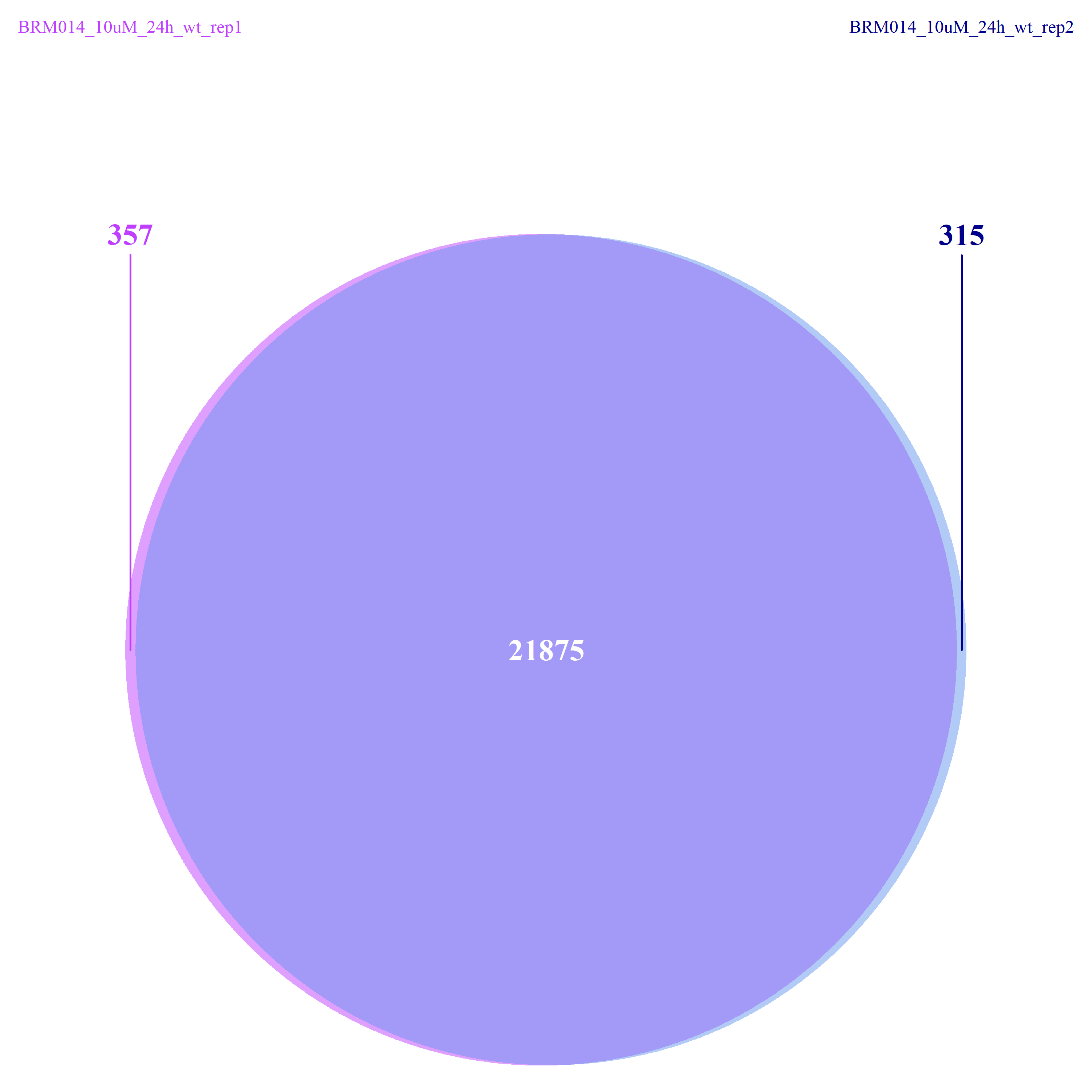
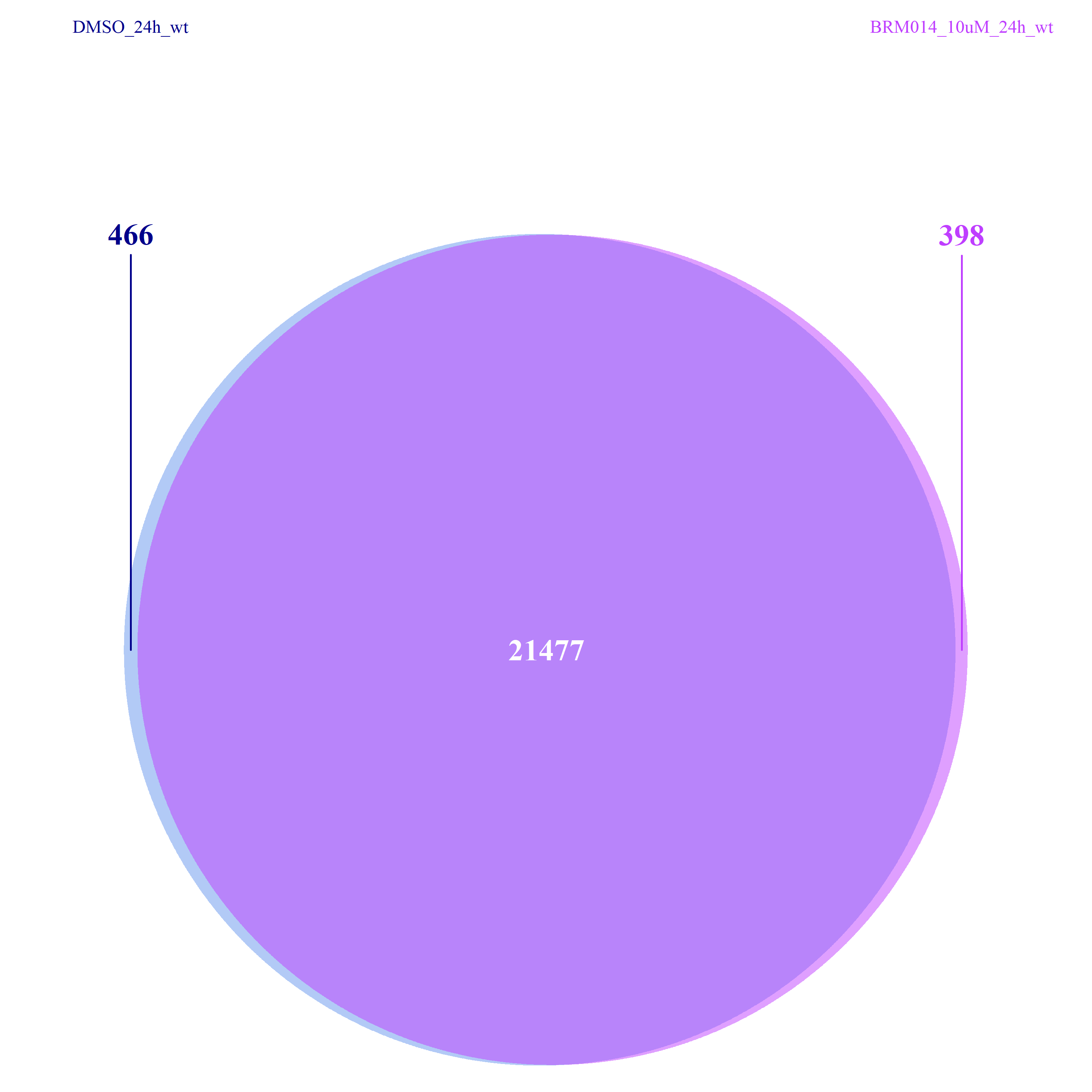
从下图可以看出,不管是组间还是组内,差异的peaks数目都不是很多了,这一点也验证了我们上面做的再全基因组范围内查看peaks的分布结果。

2020 ATAC-seq analysis