可变剪切之SUPPA2
RNA-seq高级分析之可变剪切
可变剪切之SUPPA2
SUPPA2参考资料:
https://github.com/comprna/SUPPA/wiki/SUPPA2-tutorial#differential-splicing-with-local-events
分析流程中所需要得参考基因组、注释文件、R脚本都可以在该链接中找到并下载
下面这段话引自官网,简单了解一下SUPPA2及其功能
SUPPA2 obtains the inclusion levels of AS events exploiting transcript quantification. There are different measures for isoform quantification (counts, TMM, FPKM…). We strongly recommend the use of TPM (Transcripts Per Million), because is normalized for gene length first, and then for sequencing depth. This allows direct comparison between samples (check the following video if you want to know more).
There are several tools for transcript quantification (this is an interesting review² on this matter). Each one has different pros and cons and the user is free to use the one that fits better to his requirements. We recommend to use Salmon³, because is one of the fastest methods for quantification without compromising accuracy and it also offers some other interesting options like GC bias correction or bootstrapping among others. The commands indicated here are oriented for using this tools.
(一)环境搭建
1 | conda create -n SUPPA2_3.9 python=3.9.1 |
(二)转录本定量
1、建立索引
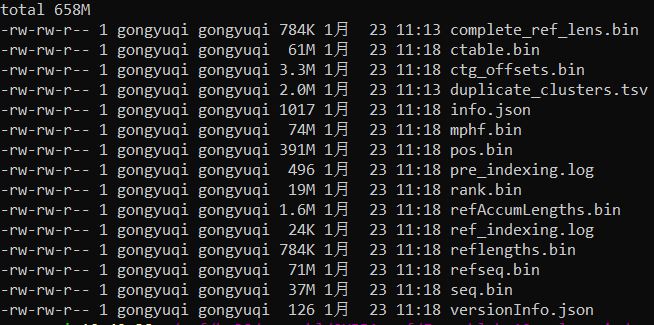
1 | salmon index -t hg19_EnsenmblGenes_sequence_ensenmbl.fasta -i Ensembl_hg19_salmon_index |
2、定量获得TPM值
(1)、运行salmon软件定量
1 | x=_1 |
展示一个样本的输出结果结构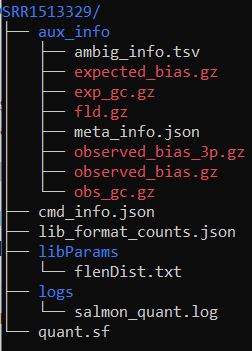
其中quant.sf文件很重要,要用于后续的分析,展示该文件部分内容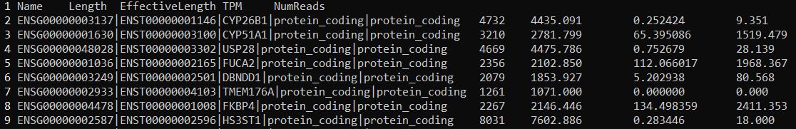
(2)、提取所有样本的TPM值并合并为一个文件
-k indicates the row used as index-f TPM值在第四列,在这里要提取每个样本的TPM值
1 | suppa_dir=/home/gongyuqi/miniconda3/envs/SUPPA2_3.9/bin/ |
查看iso_tpm.txt的内容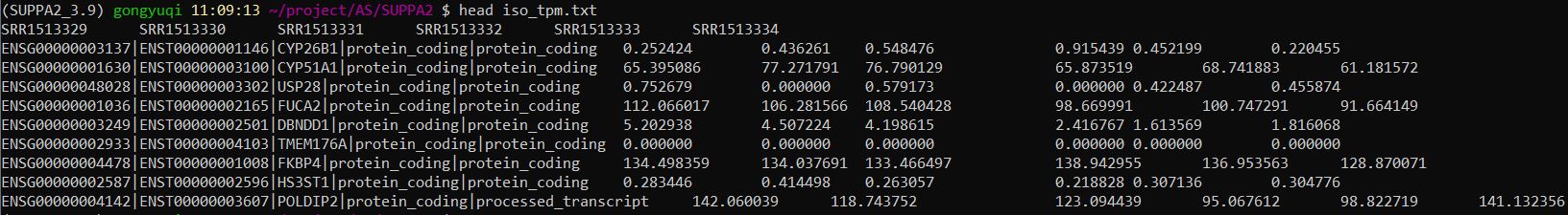
(3)、使iso_tpm.txt文件中的转录本id同下载的gtf文件id一致
运行此R脚本,会生成iso_tpm_formatted.txt文件
1 | Rscript format_Ensembl_ids.R iso_tpm.txt |
查看iso_tpm_formatted.txt的内容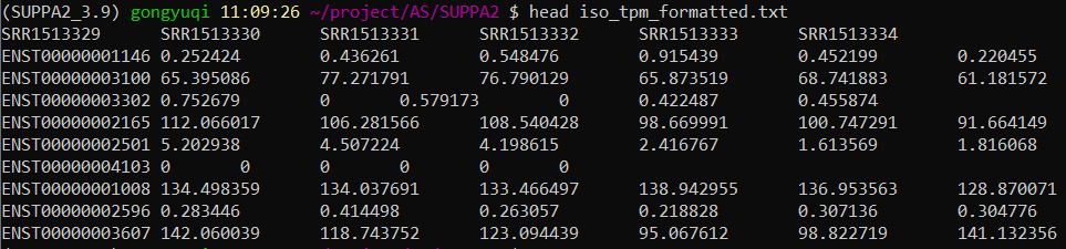
三、PSI计算
1、根据参考基因组注释文件生成可变剪切事件文件
-i GTF文件-o 输出文件前缀-e 输出文件中包含的可变剪切类型-f 输出的格式
1 | #生成ioe文件 |
结果如下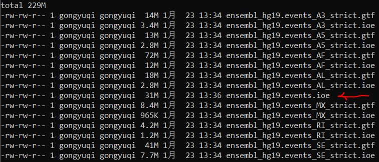
2、计算样本的PSI值
1 | cd /home/gongyuqi/project/AS/SUPPA2 |
查看结果TRA2_events.psi文件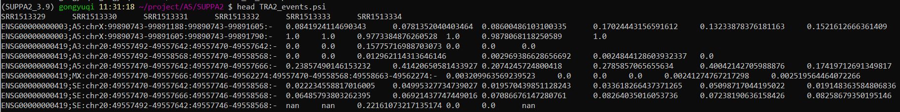
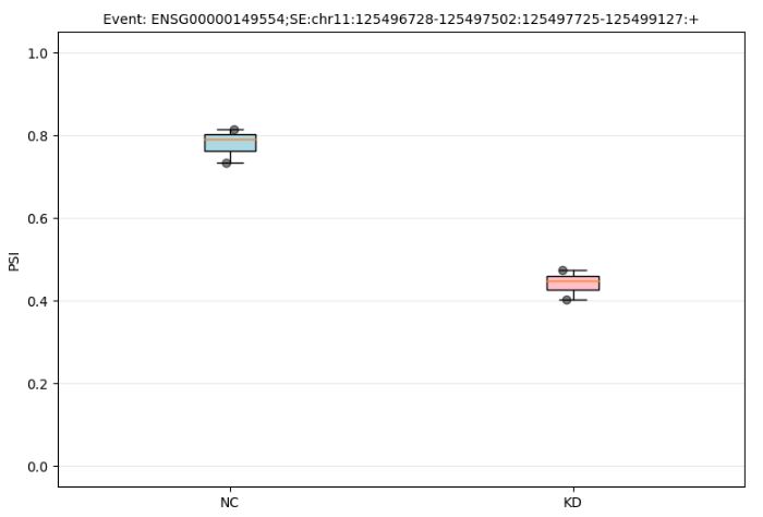
3、boxplot图可视化
-i 输入的PSI矩阵-e 需要可视化的某基因的某种可变剪切类型-g 样品按顺序分组-c 分组名称,1-3好样本为NC组,4-6号样本为KD组-o 结果输出地址
以ENSG00000149554为例进行可视化
1 | scripts_dir=/home/gongyuqi/project/AS/SUPPA2/scripts |
四、差异可变剪切分析
分组情况
negative control siRNA :SRR1513329,SRR1513330,SRR1513331
TRA2A/B siRNA :SRR1513332,SRR1513333,SRR1513334
1、分别构建两组的TPM和PSI文件
1 | $scripts_dir/split_file.R iso_tpm_formatted.txt SRR1513329,SRR1513330,SRR1513331 SRR1513332,SRR1513333,SRR1513334 TRA2_NC_iso.tpm TRA2_KD_iso.tpm -i |
2、差异分析
-m empirical 选择empirical方法-gc 基因修正--save_tpm_events 参数的添加,会多生成一个
TRA2_diffSplice_avglogtpm.tab文件,是后续火山图可视化的输入文件之一
1 | python $suppa_dir/suppa.py diffSplice -m empirical -gc -i $ioe_merge_file --save_tpm_events -p TRA2_KD_events.psi TRA2_NC_events.psi -e TRA2_KD_iso.tpm TRA2_NC_iso.tpm -o ./test/TRA2_diffSplice |
差异分析生成下列3个文件
1 | cat TRA2_diffSplice.dpsi|grep "ENSG00000149554"|less -N |
查看dpsi文件,以ENSG00000149554为例,分析结果中会显示这个基因不同的可变剪切类型在两种处理情况下的psi值及其显著性,红色箭头标记的可变剪切事件在两组中的差异是显著的(p_value<0.05)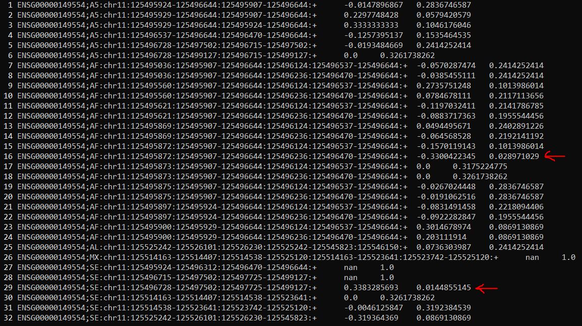
当然,上述可变剪切差异分析的结果还可以导入R中进行volcanoplot可视化分析,官网提供了具体的R脚本
可视化结果如下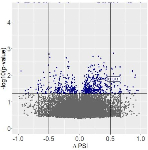
总结:
1、技术路线:salmon定量获得各个样本的TPM值——> 合并样本——> 计算PSI值——> 可变剪切差异分析
2、拿到最终的差异分析结果,提取出显著的差异可变剪切事件,写脚本将可变剪切事件的id转换成基因名,就得视觉上更友好的文件了。拿到这个文件开展后续的个性化分析。
可变剪切之SUPPA2